hi,I have some raw data samples of FM from USRP. I now want to take
their
FFT and analyze the spectrum to see whether the data that I have
captured is
valid or not. My question is that when plotting FFT in MATLAB should I
take
the range of frequencies from 0 - 10 MHz (as the signal has been shifted
to
IF of 5.75 MHz) or the range of frequencies should be 88 - 100 Mhz.
Though, No matter what range I take I always see a peak right in the
middle
of my frequency range:
e.g. if I keep the range at 0 -10 MHz, I’ll get a peak at 5.0 MHz
when I keep it at 88MHz - 108Mhz I get the peak at 98 MHz
I don’t know what you mean by the range of frequencies? I’m guessing
you’re just referring to the x-axis labels in Matlab. That would
depend on your sampling frequency after the decimation and the number
of points that you use for the FFT. Let’s say your sampling frequency
is 16Msps and you’re taking 1s of data for the FFT. Your x-axis will
look as follows:
-16000000/2:1:(16000000/2)-1 or
-samp_freq/2:samp_freq/no_samples:(samp_freq/2)-1
If you get a peak in the middle of your data, then you have a DC
offset somewhere.
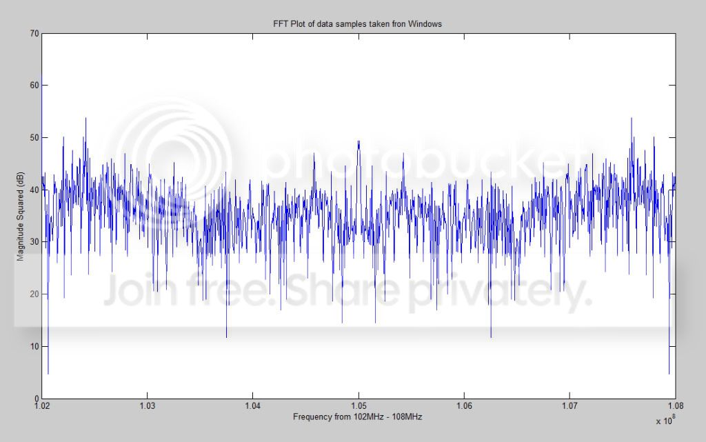
I am taking some data samples with a piece of code in Windows that takes
the
raw data samples. Now, I want to analyze the samples, whether my data is
correct or not. For this, I tune to the FM frequency of 106.2 MHz (a
radio
station) and pick some data samples.
I arbitaraily picked 956 samples and took their FFT, kept my x-axis
label
between 105 - 108 MHz and made a plot in MATLAB:
The decimation rate is 250, so my sampling frequency in this case is
64Msps/250 = 256KHz
Now, shouldn’t I be seeing a peak at 106.2 MHz? Instead at 105MHz? There
is
no station at 105MHz.
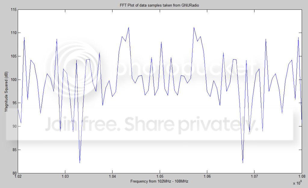
For comparison I also took some data samples from GNURadio for the same
frequency with Octave and plotted them in MATLAB:
Even here I don’t see a peak at 106.2MHz
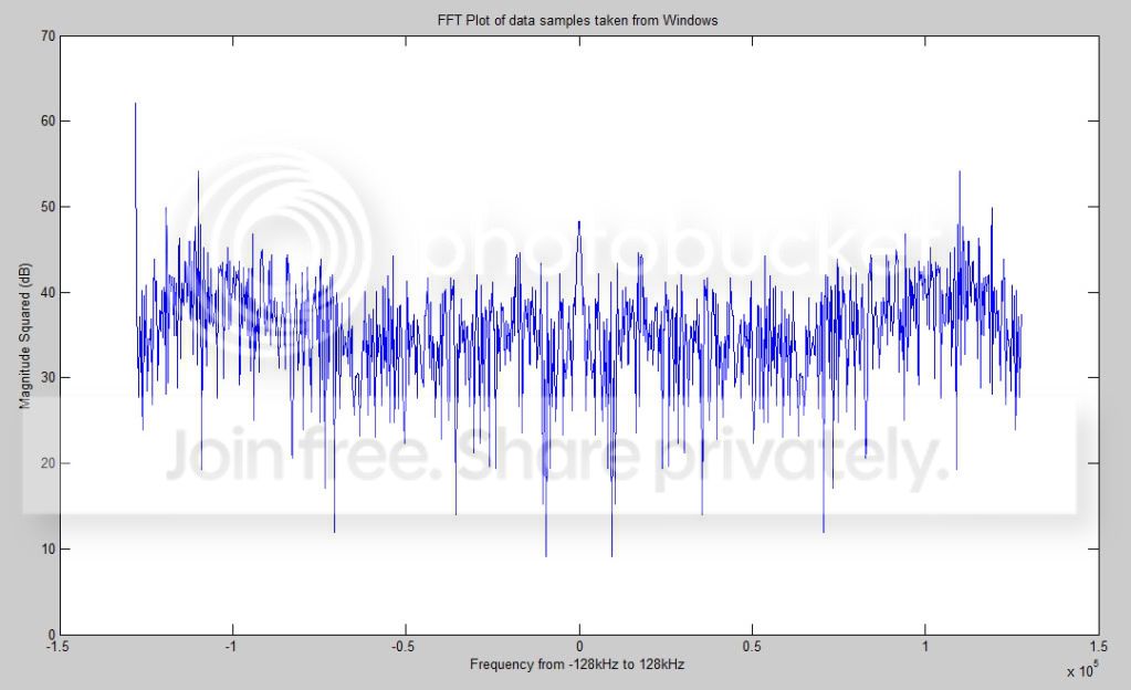
I also used the values that you told me:
-samp_freq/2:samp_freq/no_samples:(samp_freq/2)-1
as my decimation rate is 250, my sampling frequency is: 256kHz
and the no. of samples I am using is 956
so my range is: -128kHz:256kHz/956:127.999kHz
Here is the plot, again taken from Windows:
Now I don’t see any peak at 106.2MHz in any of these plots. What could
be
the problem?
You have to use usrp.tune(self.u, 0, self.subdev,106.2e6). This will
mix whatever is at 106.2MHz down to DC. set_rx_freq is used to
control the DDC in the USRP and only works from -32e6 to 32e6MHz.
The tune function first uses the mixer in the TVRX db to mix the
signal down to 5.75MHz (the TVRX db that I’m using mixes the signal
down to 44MHz). If you’re using your db, the signal gets sampled and
sits at 5.75MHz. The DDC now needs to mix it down to DC. The tune
function takes care of both of these functions for you.
Try to capture a signal by setting decimation to 250 and tuning to
106.2MHz. The result should be a signal shaped like a bell that
nearly spans the entire length of the plot.
Hi,
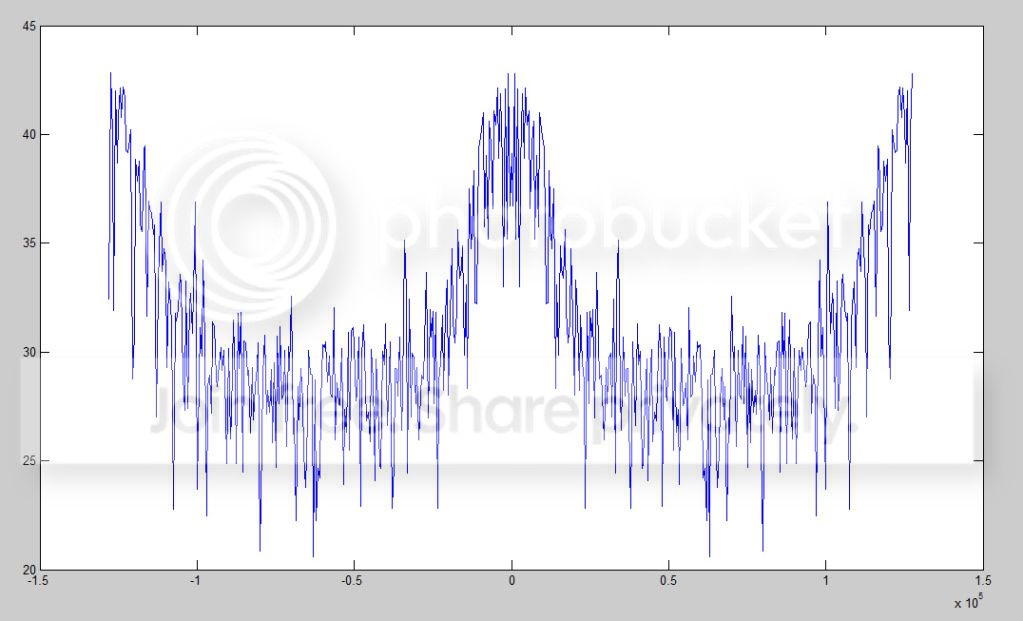
I am now getting the following plot, when I set my target_freq to 89MHz
(another radio station), with center_freq in set_rx_freq() function to
-5.75:
The decimation rate is 250 and the sampling frequency is at 256ksps.
I am getting a bell shape but it is not taking the entire length of the
plot. What could be wrong?
With a decimation of 250, your USRP will only provide you with the
samples from -128kHz to 128kHz-1. So, unless your station of interest
is very close to DC, you won’t see it on an FFT of your data. If your
signal is at an IF of 5.75MHz, you will need to sample at 16Msps in
order to digitise it.
Try an experiment. Tune your USRP to 106.2MHz (so that your radio
station now sits at DC). Set the decimation to 250
(Fs=64e6/250=256ksps). Now capture 1s of data and do a 256000 point
FFT in Matlab. You should now see a nice FM signal at DC.
You can use the usrp_wfm_rcv.py gnuradio-examples script to see what
happens in the FM band where you are.
That looks like an FM signal at DC with another FM signal about 150kHz
away. The modulating signal of the FM wave in your picture is
probably speech. If you capture another set of samples using the same
procedure, but with rock/rap/hip hop music, etc. (in other words
anything with a lot of spectral content), you should see a better bell
shape. The signal should then sit between about -50kHz and 50kHz on
your plot. FM’s maximum frequency deviation is 75KHz either way of
the carrier, so music should give you something close to that (hence
the -50kHz to 50kHz). Hope this helps.
Regards
Sebastiaan
This forum is not affiliated to the Ruby language, Ruby on Rails framework, nor any Ruby applications discussed here.